When I was TA’ing for Automata Theory, the in-browser finite-state machine creators I found tended to feel either a bit restricted or unable to generate high-quality automata images. Lo and behold, LaTeX already had a package which produced diagrams from a description.
This short guide includes some examples for creating finite state automata using LaTeX and tikz. For something more in-depth, the TikZ and PGF Manual chapter is a great reference.
Finite Automata
tikz is a great package for drawing both deterministic and nondeterministic Finite Automata. The arrows, automata, and positioning libraries used in conjunction provide all we should need.
\usepackage{tikz}
\usetikzlibrary{arrows,automata,positioning}
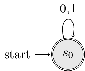
Let’s start with four examples that illustrate some of the languages regular languages can represent. The empty set can be recognized by many machines, but the final state is always an empty set.
% { }
\begin{tikzpicture}[shorten >=1pt,node distance=2cm,on grid,auto]
  \tikzstyle{every state}=[fill={rgb:black,1;white,10}]

  \node[state,initial] (s_0)  {$s_0$};

  \path[->]
  (s_0) edge  [loop above]  {0,1} ( );
\end{tikzpicture}
The natural opposite of a machine that accepts nothing is a machine which accepts everything. By the same logic as before, all automata where Q equals F will recognize this language.
% {0,1}*
\begin{tikzpicture}[shorten >=1pt,node distance=2cm,on grid,auto]
  \tikzstyle{every state}=[fill={rgb:black,1;white,10}]

  \node[state,initial,accepting] (s_0)  {$s_0$};

  \path[->]
  (s_0) edge  [loop above]  {0,1} ( );
\end{tikzpicture}
Positioning Nodes on the Grid
Now that we’ve seen the two languages which can be expressed with a single state, we turn our focus to those which require two or more states.
The next two languages represent ε and {0,1}+. Respectively these correspond to “the language of strings containing nothing” and “the language of strings containing something”. From these images it is also worth noticing that they are inverses of one another.
These examples use a position parameter to show that s_1 should be positioned to the right of=s_0.
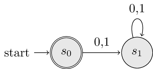
% { \epsilon }
\begin{tikzpicture}[shorten >=1pt,node distance=2cm,on grid,auto]
  \tikzstyle{every state}=[fill={rgb:black,1;white,10}]

  \node[state,initial,accepting]  (s_0)                 {$s_0$};
  \node[state]                    (s_1) [right of=s_0]  {$s_1$};

  \path[->]
  (s_0) edge                node {0,1}  (s_1)
  (s_1) edge  [loop above]  node {0,1}  ();
\end{tikzpicture}
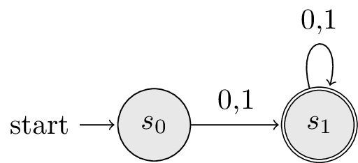
% { 0,1 }+
\begin{tikzpicture}[shorten >=1pt,node distance=2cm,on grid,auto]
  \tikzpicture{every state}=[fill={rgb:black,1;white,10}]

  \node[state,initial,accepting]  (s_0)                 {$s_0$};
  \node[state]                    (s_1) [right of=s_0]  {$s_1$};

  \path[->]
  (s_0) edge                node {0,1}  (s_1)
  (s_1) edge  [loop above]  node {0,1}  ();
\end{tikzpicture}
Arcs as Edges
As automata grow more complicated, it’s beneficial to have control over placement of both the nodes and the edges.
This example (Figure 1.4 from Sipser (3rd Edition)) uses right of= for positioning the nodes, but edges on the path all either loop above a node or bend left.
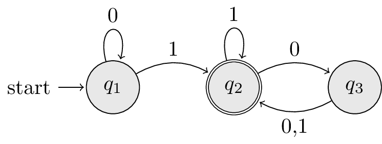
\begin{tikzpicture}[shorten >=1pt,node distance=2cm,on grid,auto]
  \tikzstyle{every state}=[fill={rgb:black,1;white,10}]

    \node[state,initial]   (q_1)                    {$q_1$};
    \node[state,accepting] (q_2)  [right of=q_1]    {$q_2$};
    \node[state]           (q_3)  [right of=q_2]    {$q_3$};

    \path[->]
    (q_1) edge [loop above] node {0}    (   )
          edge [bend left]  node {1}    (q_2)
    (q_2) edge [bend left]  node {0}    (q_3)
          edge [loop above] node {1}    (   )
    (q_3) edge [bend left]  node {0,1}  (q_2);
\end{tikzpicture}
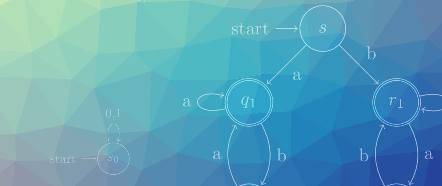
Finally, this example (Figure 1.12 From Sipser (3rd Edition)) puts together all of the pieces seen so far: positioning nodes on the grid, loops, and directed edges.
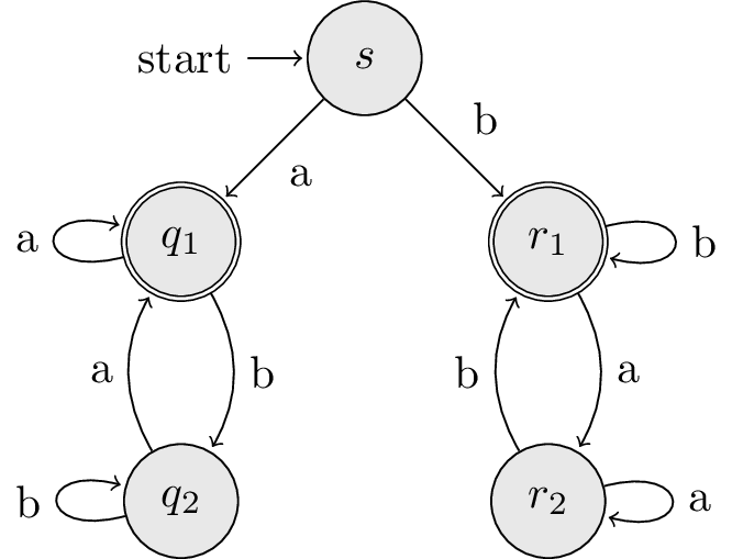
\begin{tikzpicture}[shorten >=1pt,node distance=2cm,auto]
  \tikzstyle{every state}=[fill={rgb:black,1;white,10}]

  \node[state,initial]   (s)                      {$s$};
  \node[state,accepting] (q_1) [below left of=s]  {$q_1$};
  \node[state]           (q_2) [below of=q_1]     {$q_2$};
  \node[state,accepting] (r_1) [below right of=s] {$r_1$};
  \node[state]           (r_2) [below of=r_1]     {$r_2$};

  \path[->]
  (s)   edge              node {a} (q_1)
        edge              node {b} (r_1)
  (q_1) edge [loop left]  node {a} (   )
        edge [bend left]  node {b} (q_2)
  (q_2) edge [loop left]  node {b} (   )
        edge [bend left]  node {a} (q_1)
  (r_1) edge [loop right] node {b} (   )
        edge [bend left]  node {a} (r_2)
  (r_2) edge [loop right] node {a} (   )
        edge [bend left]  node {b} (r_1);
\end{tikzpicture}