Quick Overview
I stumbled upon a 2010 paper by Vanathi Gopalakrishnan, Jonathan L. Lustgarten, Shyam Visweswaran, and Gregory F. Cooper titled: “Bayesian rule learning for biomedical data mining.”1
Their idea was to develop an algorithm for learning probabilistic/logical rules, but with ten years of hindsight available to me, it seemed to anticipate methods now developed in “explainable or interpretable machine learning.”2 The authors describe (1) learning Bayesian networks using a modified K2 structure learning approach, then (2) extracting rules from the conditional probability tables.
The pattern of “fit a model” and then “apply post-hoc analysis” to tame complexity is now a staple of machine learning explainability. My goal in this post is to interpret the paper in this slightly different context, and suggest some extensions.
I’ll assume that you already know a little about Bayesian networks and factorized probability distributions. Since inference is hard in the general case,3 our goal is to learn something about our data using Bayesian networks without having to run inference.
Interpreting the BRL pseudocode
Gopalakrishnan et al. developed their “Bayesian Rule Learning” (BRL) algorithm in two parts, starting on page three. The first part is a structure scoring approach based on a modified version of the K2 criteria. This provides an estimate of the data likelihood given a model.4
With a scoring method in place, lines 1-9 use beam search to find a Bayesian network structure using the modified K2 criteria for scroing, with the "for-each" (line 8) possibly providing some input via variable ordering. Otherwise this makes local changes to the structures so long as the "maximum number of parents" constraint is not violated, places in-progress structures back on the beam, and records structures that cannot be improved onto a final priority queue. Finally, line 10 converts the best structure into rules.
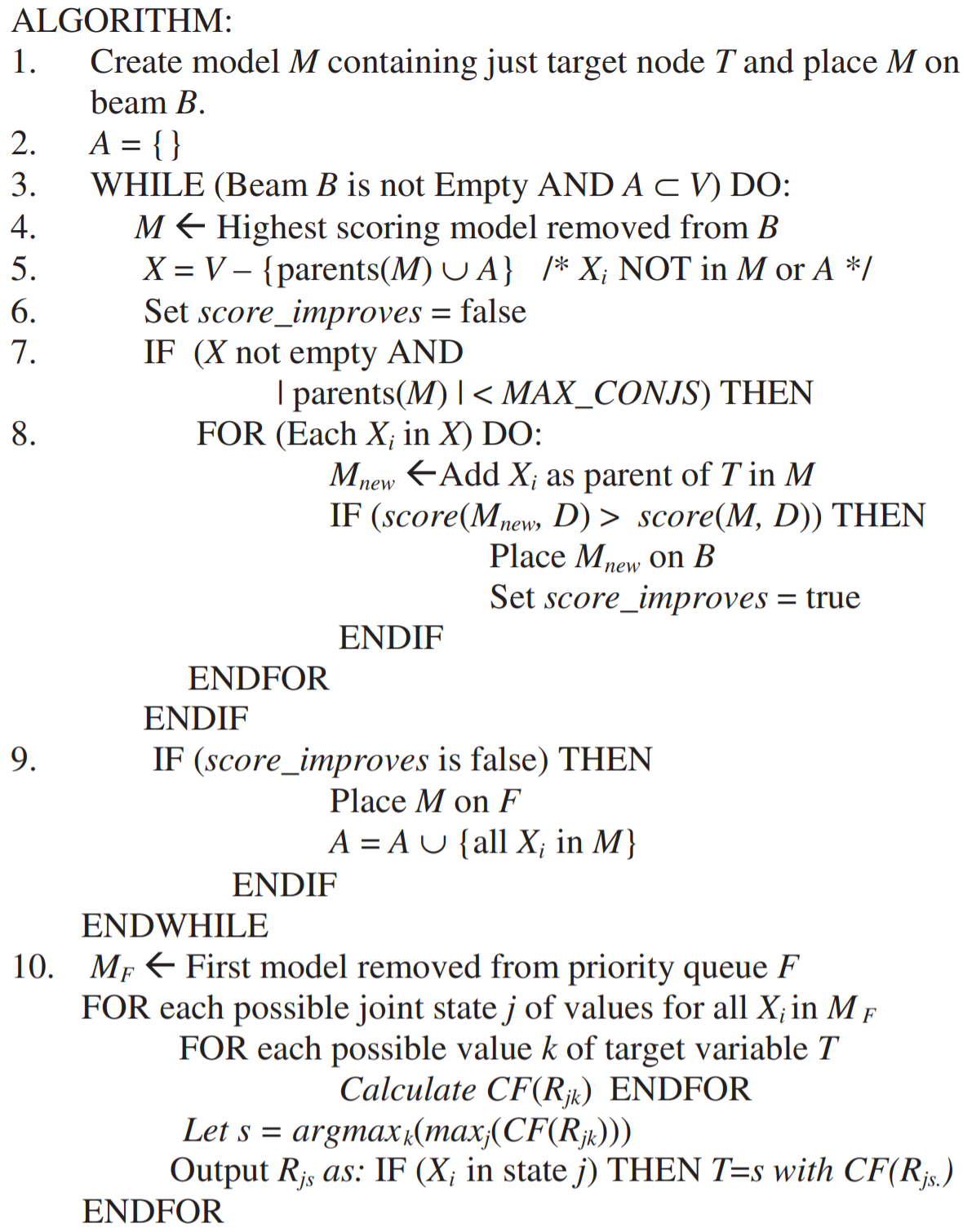
For easier viewing, I made a rough transcription of the algorithm into a Julia-like syntax:
1
2
3
4
5
6
7
8
9
10
11
12
13
14
15
16
17
18
19
20
21
22
23
24
25
26
B = Beam(1000)([BayesNet(T)])       # Initialize width-1000 Beam with a BayesNet containing T
A = Set()                           # 𝐴 is a subset of variables 𝑉 containing Xᵢ in final structures
F = PriorityQueue()                 # 𝐹 contains final structures that cannot be improved further

while (!isempty(B) && A ⊂ V)
  M = maximum(B)                    # Highest scoring model removed from 𝐵
  X = setdiff(V, A ∪ parents(M))    # Xᵢ not in 𝑀 or 𝐴

  score_improves = false

  if (!isempty(X) && size(parents(M) < MAX_CONJS))
    for Xᵢ in X
      Mₙ = add_parent(M, Xᵢ, T)     # Add Xᵢ as a parent of T in M

      if score(Mₙ, D) > score(M, D)
        push!(B, Mₙ)                # Place the new model Mₙ on the Beam
        score_improves = true
      end
    end
  end

  if !score_improves
    push!(M, F)                       # Place 𝑀 on 𝐹
    A = A ∪ M.variables
  end
end
Since line 8 (line 13 in my transcription) exclusively adds variables as parents of the target \(\mathit{T}\), it should only be possible to produce structures like the following:


Line 10 occurs independently from the rest of the listing. It removes the best model from the priority queue \(\mathit{F}\) and uses the joint distribution over the variables to create IF/THEN rules.
1
2
3
4
5
6
7
8
9
10
model = first(F)                    # First model removed from priority queue 𝐹
for Xᵢ ∈ model
  for j ∈ Xᵢ                        # Each joint state of values
    for k ∈ T
      CF(R[j][k])
    end
    s = argmaxₖ(maxⱼ(CF(R[j][k])))
    println("IF ($Xᵢ = $j) THEN ($T = $s); $(CF(R[j][s]))")
  end
end
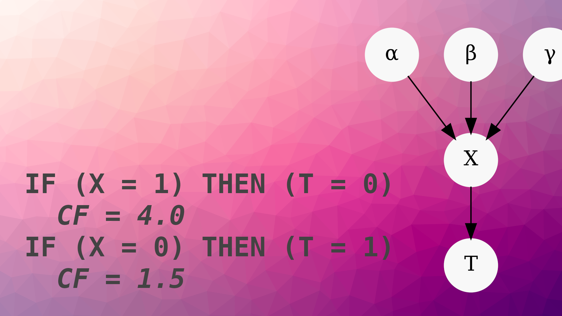
But as suggested in Figure 3 of the paper, it’s fairly easy to see how this works using an example. Consider the following two-variable model with binary variables and these conditional probability tables:

$$ \begin{split} P(X = 0) = 0.7 \cr P(X = 1) = 0.3 \cr\cr P(T = 0 \mid X = 0) = 0.2 \cr P(T = 1 \mid X = 0) = 0.8 \cr P(T = 0 \mid X = 1) = 0.6 \cr P(T = 1 \mid X = 1) = 0.4 \end{split} $$
The “rule extraction” portion of the algorithm can produce four rules. The confidence factor (CF) is the likelihood ratio for and against an outcome \(T\) when presented with evidence \(X = x\):
  IF (X = 0) THEN T = 0
    CF = 0.25                     # 0.25 = 0.2 / 0.8
  IF (X = 0) THEN T = 1
    CF = 4.0                      # 4.00 = 0.8 / 0.2
  IF (X = 1) THEN T = 0
    CF = 1.5                      # 1.50 = 0.6 / 0.4
  IF (X = 1) THEN T = 1
    CF = 0.67                     # 0.67 ≈ 0.4 / 0.6
Another suggestion in figure 3 is to prune the cases with lowest confidence given the same evidence:5
- IF (X = 0) THEN T = 0
-   CF = 0.25
  IF (X = 0) THEN T = 1
    CF = 4.0
  IF (X = 1) THEN T = 0
    CF = 1.5
- IF (X = 1) THEN T = 1
-   CF = 0.67
Which says that the most likely situation is for the values of \(X\) and \(T\) to be opposites of one another:
  IF (X = 0) THEN T = 1
    CF = 4.0
  IF (X = 1) THEN T = 0
    CF = 1.5
Or:
T ⟺ ¬X
It’s a lossy way to describe the Bayesian network, but we learned something about what happens in general without having to invoke variable elimination, factor graphs, message passing, or any other machinery.
The sum of these two parts forms the “Bayesian Rule Learning” algorithm. But thinking a bit more generally, structure learning and rule extraction are independent, and a host of different knobs are available in each now that we’ve seen the basic layout. For instance, we could replace the structure learning portion with any off-the-shelf method. Furthermore, extracting rules from arbitrary structures to learn how variables are related can give us a constrained association rule mining technique.
The next few sections present an implementation and some suggestions for how to apply it.
Implementing Bayesian Rule Learning as a Python package
I implemented the rule extraction portion as a Python package; code is on my GitHub (https://github.com/hayesall/bn-rule-extraction/),
Currently it’s designed as an explainability method for the
pomegranate BayesianNetwork format.
But it would be fairly straightforward to extend this if you wanted to use the rules directly
for classification.
A copy can be installed locally with pip, or there are Google Colab links for some Jupyter notebooks accompanying the discussion here.
pip install git+https://github.com/hayesall/bn-rule-extraction.git
Bayesian Rules for Deciding when People Play Tennis
| Open Notebook in Colab | View Notebook on GitHub |
|---|---|
 |
You’re walking your dog past the YMCA tennis courts, because your dog likes going on walks every day and thinks the tennis courts smell interesting. But you notice the courts are only occupied about half the time. Not having anything better to do, you start collecting some data on court occupation and weather each day.6
| PlayTennis | Outlook | Temperature | Humidity | Wind | |
|---|---|---|---|---|---|
| 0 | no | sunny | hot | high | weak |
| 1 | no | sunny | hot | high | strong |
| 2 | yes | overcast | hot | high | weak |
| ... | ... | ... | ... | ... | ... |
| 11 | yes | overcast | mild | high | strong |
| 12 | yes | overcast | hot | normal | weak |
| 13 | no | rain | mild | high | strong |
from bayes_rule_extraction import ordinal_encode, print_rules
from pomegranate import BayesianNetwork
import pandas as pd

data = pd.read_csv("https://raw.githubusercontent.com/hayesall/bn-rule-extraction/main/toy_decision.csv")
data
Naive Bayes for Tennis
We’ll want to ordinal encode the data before handing it to pomegranate, and we’ll want a mapping
between category codes back into an easy-to-read representation later.
ordinal_encode is a small helper function around the
scikit-learn OrdinalEncoder object, which returns a float32 numpy array and a dictionary
mapping the encoded format back to the string format.
encoded, mapping = ordinal_encode(data.columns, data)
encoded
  array([[0., 2., 1., 0., 1.],
         [0., 2., 1., 0., 0.],
         [1., 0., 1., 0., 1.],
         ...,
         [1., 0., 2., 0., 0.],
         [1., 0., 1., 1., 1.],
         [0., 1., 2., 0., 0.]], dtype=float32)
Naive Bayes assumes that the variables are conditionally independent given the target. We’ll represent this by passing a fixed structure where all of the variables have PlayTennis (the variable with index 0) as a parent.7

naive_model = BayesianNetwork.from_structure(
    encoded_data,
    structure=((), (0,), (0,), (0,), (0,)),
    state_names=data.columns,
)
The network is backwards to a sensible causal story (surely playing tennis doesn’t cause rain), and the influence directions are opposite to the one suggested by the BRL algorithm.
print_rules(naive_model, data.columns, mapping)
  Probabilities:
  - PlayTennis
      P( PlayTennis = no ) = 0.36
      P( PlayTennis = yes ) = 0.64

  IF (PlayTennis = no) THEN (Outlook = sunny)
      CF = 1.50
  IF (PlayTennis = no) THEN (Humidity = high)
      CF = 4.00
  IF (PlayTennis = yes) THEN (Humidity = normal)
      CF = 2.00
  IF (PlayTennis = no) THEN (Wind = strong)
      CF = 1.50
  IF (PlayTennis = yes) THEN (Wind = weak)
      CF = 2.00
Nonetheless, the rules tell us something about how the each outcome is related to potential conditions:
- “On days when tennis is played, the humidity is probably normal.”
- “On days when tennis is played, the wind is probably weak.”
- “On days when tennis is NOT played, the humidity is probably high.”
Structure Learning + Rule Extraction for the Binary Classification Case
A simple constraint would be to prevent PlayTennis from being the parent of any other node.
We can encode this using the exclude_edges parameter, and passing a list of tuples representing
forbidden edges: (0, 1), (0, 2), (0, 3), (0, 4).

excluded_edges = [
  tuple([0, i]) for i in range(1, len(data.columns))
]

binary_model = BayesianNetwork().from_samples(
  encoded_data,
  exclude_edges=excluded_edges,
  state_names=data.columns,
)
The portion we’re interested in: \(\text{Humidity} \rightarrow \text{PlayTennis}\), is almost identical to our motivating example. Extracting rules from this network shows that high humidity and tennis playing tend to be opposites:
IF (Humidity = high) THEN (PlayTennis = no)
    CF = 1.33
IF (Humidity = normal) THEN (PlayTennis = yes)
    CF = 6.00
Using a structure that maximizes “PlayTennis” accuracy
There’s one structure I want to highlight—where Outlook and Wind are parents of our target
variable—similar to the kind of structures the authors suggested. I stumbled into this structure while searching
for cases with maximum leave-one-out-cross-validation accuracy for predicting PlayTennis:

known_structure_model = BayesianNetwork.from_structure(
    encoded_data,
    structure=((1, 4), (), (), (2,), ()),
    state_names=data.columns,
)
The causal interpretation still seems tenuous—it seems like a sunny or overcast outlook should affect the temperature. But it also seems overly optimistic to expect causal explanations from the fictional world this data was drawn from.
This structure is a case where multiple conditions
affect an outcome since Outlook and Wind influence PlayTennis. Running the rule extraction
method produces some interesting rules:
IF (Outlook = overcast ^ Wind = strong) THEN (PlayTennis = yes)
	CF = inf
IF (Outlook = overcast ^ Wind = weak) THEN (PlayTennis = yes)
	CF = inf
IF (Outlook = rain ^ Wind = strong) THEN (PlayTennis = no)
	CF = inf
IF (Outlook = rain ^ Wind = weak) THEN (PlayTennis = yes)
	CF = inf
IF (Outlook = sunny ^ Wind = strong) THEN (PlayTennis = no)
	CF = 1.00
IF (Outlook = sunny ^ Wind = strong) THEN (PlayTennis = yes)
	CF = 1.00
IF (Outlook = sunny ^ Wind = weak) THEN (PlayTennis = no)
	CF = 2.00
Let’s start with a case I’ll call “indeterminate evidence.” Two rules contain the same observations, but reach opposite conclusions with equal confidence: “On sunny, windy days—playing tennis or not is equally likely.”
IF (Outlook = sunny ^ Wind = strong) THEN (PlayTennis = no)
	CF = 1.00
IF (Outlook = sunny ^ Wind = strong) THEN (PlayTennis = yes)
	CF = 1.00
The conditional probability tables result from the training data, and when we revisit the data it’s obvious why this occurs: we observed both situations.8
   PlayTennis Outlook     Wind
------------------------------
1          no   sunny   strong
10        yes   sunny   strong
The opposite problem occurs when we have infinite confidence in the outcomes:
IF (Outlook = overcast ^ Wind = strong) THEN (PlayTennis = yes)
	CF = inf
“Infinite confidence” occurs due to a divide-by-zero runtime exception when comparing the likelihood of events with no counterexamples. Again we can look at the training data and see this occurs because we have two examples where the outlook is overcast and the wind is strong; and our imaginary users played tennis on both days:
   PlayTennis   Outlook    Wind
-------------------------------
6         yes  overcast  strong
11        yes  overcast  strong
?          no  overcast  strong    <-- never observed in the training data
Taken together, “indeterminate evidence” or “infinite confidence” could suggest places in the observation space where the decision is deterministic (infinite confidence in an outcome), or the decision is random (equal likelihood).9 This could also be a limitation with likelihood ratios, and the authors hinted that other metrics (e.g. support) could be more appropriate in specific settings.
The next section applies the method to a slightly more real-world dataset.
Bayesian Rule Extraction to Explain Income from Census Data
| Open Notebook in Colab | View Notebook on GitHub |
|---|---|
|
Now we’ll turn our focus toward applying the “Bayesian Rule Learning” algorithm to a more-realistic Adult dataset, which is a common benchmark for interpretable or fair methods (I adapted some of the setup here from the InterpretML documentation for the Explainable Boosting Machine—used under the MIT License).
This follows the standard binary classification problem. The goal is to predict whether a person made more/less than $50,000 using attributes like “Age,” “Education,” “MaritalStatus,” etc. To simplify, I chose to exclude missing values and continuous attributes here.
from bayes_rule_extraction import ordinal_encode, print_rules
from pomegranate import BayesianNetwork
import pandas as pd

data = pd.read_csv(
    "https://archive.ics.uci.edu/ml/machine-learning-databases/adult/adult.data",
    header=None,
)
data.columns = [
    "Age", "WorkClass", "fnlwgt", "Education", "EducationNum",
    "MaritalStatus", "Occupation", "Relationship", "Race", "Gender",
    "CapitalGain", "CapitalLoss", "HoursPerWeek", "NativeCountry", "Income"
]

data.drop(["Age", "fnlwgt", "EducationNum", "CapitalGain", "CapitalLoss", "HoursPerWeek"], axis=1, inplace=True)
data.replace(" ?", pd.NA, inplace=True)
data.dropna(inplace=True)
data
| WorkClass | Education | MaritalStatus | Occupation | Relationship | Race | Gender | NativeCountry | Income | |
|---|---|---|---|---|---|---|---|---|---|
| 0 | State-gov | Bachelors | Never-married | Adm-clerical | Not-in-family | White | Male | United-States | <=50K |
| 1 | Self-emp-not-inc | Bachelors | Married-civ-spouse | Exec-managerial | Husband | White | Male | United-States | <=50K |
| 2 | Private | HS-grad | Divorced | Handlers-cleaners | Not-in-family | White | Male | United-States | <=50K |
| 3 | Private | 11th | Married-civ-spouse | Handlers-cleaners | Husband | Black | Male | United-States | <=50K |
| 4 | Private | Bachelors | Married-civ-spouse | Prof-specialty | Wife | Black | Female | Cuba | <=50K |
| ... | ... | ... | ... | ... | ... | ... | ... | ... | ... |
| 32556 | Private | Assoc-acdm | Married-civ-spouse | Tech-support | Wife | White | Female | United-States | <=50K |
| 32557 | Private | HS-grad | Married-civ-spouse | Machine-op-inspct | Husband | White | Male | United-States | >50K |
| 32558 | Private | HS-grad | Widowed | Adm-clerical | Unmarried | White | Female | United-States | <=50K |
| 32559 | Private | HS-grad | Never-married | Adm-clerical | Own-child | White | Male | United-States | <=50K |
| 32560 | Self-emp-inc | HS-grad | Married-civ-spouse | Exec-managerial | Wife | White | Female | United-States | >50K |
Again, we’ll ordinal-encode the values:
encoded, mapping = ordinal_encode(data.columns, data)
encoded
  array([[ 5.,  9.,  4., ...,  1., 38.,  0.],
         [ 4.,  9.,  2., ...,  1., 38.,  0.],
         [ 2., 11.,  0., ...,  1., 38.,  0.],
         ...,
         [ 2., 11.,  6., ...,  0., 38.,  0.],
         [ 2., 11.,  4., ...,  1., 38.,  0.],
         [ 3., 11.,  2., ...,  0., 38.,  1.]], dtype=float32)
Unconstrained Structure Learning
As humans, we tend to have a lot of prior knowledge about how we expect the world to work. Unfortunately, it’s rarely obvious what knowledge needs applying until we do some basic exploration. We’ll start with a let’s see what happens attitude by fitting parameters and a structure without prior knowledge:
unconstrained_model = BayesianNetwork().from_samples(
    encoded_data,
    state_names=data.columns,
)

Parts of this might look reasonable: the structure shows a relationship between Income and Occupation, and a relationship between Occupation and Education. If Income is still the target we’re interested in, we see influences between Relationship, Gender, and Occupation. Each of these can be explored separately (the intersection of gender, race, family structure—and their effects in combination on economic opportunities in the United States is a massive topic that I cannot hope to fully discuss here).
But similar to the Naive Bayes case from the “Tennis” example, the extracted rules are a little difficult to
interpret since Income is the root of the network, meaning the variable cannot occur after a THEN.
But also similar to the “Tennis” example, this might be enough to hint at some likely events, such as income
tending to be higher for people identified as husbands.
IF (Income > 50,000) THEN (Relationship = Husband)
    CF = 3.10
This also finds some cases where conditional influences are almost perfectly correlated, such as an observation that “husbands are married.”
IF (Relationship = Husband ^ Gender = Female) THEN (MaritalStatus = Married-civ-spouse)
    CF = inf
IF (Relationship = Husband ^ Gender = Male) THEN (MaritalStatus = Married-civ-spouse)
    CF = 1383.67
This might also be a situation where rule extraction can help reveal special cases (or mistakes) that occur during data collection. I’d previously used this dataset, but this is the first time I noticed situations where: “a husband is female,” and “a wife is male.”10
| WorkClass | Education | MaritalStatus | Occupation | Relationship | Race | Gender | NativeCountry | Income | |
|---|---|---|---|---|---|---|---|---|---|
| 575 | Private | Bachelors | Married-civ-spouse | Exec-managerial | Wife | White | Male | United-States | >50K |
| 7109 | Private | HS-grad | Married-civ-spouse | Sales | Husband | White | Female | United-States | <=50K |
Now that we’ve seen an unconstrained version, we’ll iterate to answer our question about Income.
Adding constraints to guide the structure learning
Since we’re interested in “Income,” it could make sense to require: “Income cannot be the parent of any node.”
This might help with explainability, but a causal interpretation may still be incorrect. Imagine modifying the value of one variable and observing what happens, such as an influence between ‘Income’ and ‘Education.’ We might expect something like ‘people with some college credits earn more than people with a high school education alone,’ but it’s also possible that high-wage earners have better opportunities to continue their education and earn professional degrees.
We might observe such conditional influences when observing data over time, but here we’re working with a snapshot at a specific point.
Again we’ll enforce this through excluding specific edges:
excluded_edges = [tuple([8, i]) for i in range(len(data.columns)-1)]

model = BayesianNetwork().from_samples(
    encoded,
    exclude_edges=excluded_edges,
    state_names=data.columns,
)

This tends to produce networks rooted at “MaritalStatus,” and highlights “Relationship” and “Education” influencing “Income.” The differences are pretty stark when contrasting people with a high school education against those with professional degrees.
IF (Education = HS-grad ^ Relationship = Husband) THEN (Income <= 50,000)
    CF = 2.13
IF (Education = HS-grad ^ Relationship = Not-in-family) THEN (Income <= 50,000)
    CF = 20.97
IF (Education = HS-grad ^ Relationship = Other-relative) THEN (Income <= 50,000)
    CF = 38.33
Phrased another way: at the low and high ends of education, relationship status doesn’t appear to make any difference in income.
IF (Education = Doctorate ^ Relationship = Husband) THEN (Income > 50,000)
    CF = 5.13
IF (Education = Doctorate ^ Relationship = Not-in-family) THEN (Income > 50,000)
    CF = 1.23
IF (Education = Doctorate ^ Relationship = Other-relative) THEN (Income > 50,000)
    CF = inf
Between the extreme ends, the story seems a bit more nuanced.
For example, it appears that people with an associate’s degree (or vocational training) are slightly more likely to make over $50,000 if they are also married:
IF (Education = Assoc-acdm ^ Relationship = Wife) THEN (Income > 50,000)
    CF = 1.12
IF (Education = Assoc-voc ^ Relationship = Wife) THEN (Income > 50,000)
    CF = 1.48
This also seems to highlight cases where people with a higher education but less-consistent living arrangements—such as people in a household with bachelors degrees that are not living with their immediate family members—earn less:
IF (Education = Bachelors ^ Relationship = Not-in-family) THEN (Income <= 50,000)
    CF = 4.80
IF (Education = Bachelors ^ Relationship = Other-relative) THEN (Income <= 50,000)
    CF = 12.67
Ideas and Further Thoughts
I’ve found this approach to be pretty helpful in some health informatics problems I work on, and more broadly I suspect this could help reveal deterministic paths within uncertain models, shed light on cases where domain expertise or more data are required, or perhaps reveal “bugs” in the data where a value was incorrectly recorded.
Explaining Bayesian networks is an interesting topic in itself, see the paper I wrote with Athresh, Harsha, and others on extracting qualitative influence statements, and some of the Starling Lab projects.
-
Vanathi Gopalakrishnan, Jonathan L. Lustgarten, Shyam Visweswaran, Gregory F. Cooper, Bayesian rule learning for biomedical data mining, Bioinformatics, Volume 26, Issue 5, 1 March 2010, Pages 668–675, https://doi.org/10.1093/bioinformatics/btq005 ↩
-
Christoph Molnar’s “Interpretable Machine Learning” book (and others) tend to distinguish between inherently interpretable models and post-processing to explain an uninterpretable model. The chapter on “Decision Rules” and “Bayesian Rule Lists” have some overlap with what I’m discussing here. ↩
-
How complicated? The last author on this paper—Gregory F. Cooper—proved that exact inference is NP-hard for general Bayesian networks. See: “The computational complexity of probabilistic inference using bayesian belief networks,” https://doi.org/10.1016/0004-3702(90)90060-D ↩
-
Briefly, K2 is another “search and score” structure learning method where a user defines a variable ordering and the search proceeds with one step lookahead by exploring the frontier of remaining variables that have not been used yet. See: Gregory F. Cooper and Edward Herskovits, “A Bayesian Method for the Induction of Probabilistic Networks from Data.” In Machine Learning 1992. https://doi.org/10.1007/BF00994110 ↩
-
The algorithm listing introduces a variable
srepresentingargmax(max(CF(R))): the index of the rule with maximum confidence. Therefore if you’re following the “letter of the algorithm” then pruning should not be necessary since you’ll always print the one with maximum confidence, but recasting this step as “show everything and prune” has some potential benefits I’ll describe later. Briefly: the authors suggest that multiple pruning methods are valid depending on what metrics you’re interested in, such as pruning rules with low likelihood ratios, or those with low support. ↩ -
Tom Mitchell wasn’t specific on where this data came from, but people that I’ve talked to generally seem to assume it’s fictional. However, the book does say that each observation should be interpreted as being on a Saturday—perhaps to avoid the problem where weather on consecutive days would be highly correlated. See section 3.4.2 (page 59 in Alexander’s edition). Tom M. Mitchell. McGraw Hill. (1997). 3.4.2. In “Machine Learning.” ISNB: 9781259096952 ↩
-
In the listing, this is enforced by passing “((), (0,), (0,), (0,), (0,))” as the structure parameter. The tuple-of-tuples is pomegranate’s representation where there is a tuple for each node, and the integers in a particular tuple represent the parents of that node. Therefore, “((), (0,), (0,), (0,), (0,))” tells us that we have a 5-variable Bayesian Network where variable-0 has no parents, and all other nodes have variable-0 as a parent. ↩
-
There’s an analogy we can make to decision tree induction. Usually when we learn decision trees, we greedily follow a path based on entropy or gini coefficients. We could observe what happens when introducing a third variable to give us a pure sample, but that can sometimes be a slippery slope into overfitting. ↩
-
Yes, of course a third option exists. This could simply be a signal that we don’t have enough data for these cases, in which we should consult experts for advice, or invoke constraints to better guide the learning problem. ↩
-
I spent some time plugging queries into Google Scholar to see if anyone else had noticed this. Even searching broadly with queries like “adult dataset female husband” or “adult dataset male wife” didn’t seem to reveal anything. ↩